6.2 Flux across an LCS
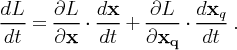
From the previous page, recall that
![]()
where here we have indicated the explicit functional dependencies of each variable. The derivative of L with time gives
|
| (16) |
For the spatial gradient of L we have,
|
| (17) |
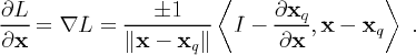
However, since xq is the point on the LCS closest to point x, then the vector x - xq must be normal to the LCS, which implies that
|
| (18) |
because the closest point on the LCS, xq,
does not change when the point x is
varied in the direction normal to the curve. As an technical point, Eq. (18) is really
only guaranteed to hold over an open neighborhood containing the LCS, within which
each point x has a unique and
well-defined xq.
This open neighborhood, which we will denote
![]() ,
always exists because the LCS is a smooth curve, and hence its curvature is finite,
implying that there always exists an open set around the LCS such that
each x in
this open set has a unique xq.
That is, since there are no kinks or discontinuities on the LCS, there always exists
an open set
,
always exists because the LCS is a smooth curve, and hence its curvature is finite,
implying that there always exists an open set around the LCS such that
each x in
this open set has a unique xq.
That is, since there are no kinks or discontinuities on the LCS, there always exists
an open set
![]() containing the LCS such that for any point
containing the LCS such that for any point
![]() ,
there is a unique point xq on
the LCS which is closer to x than any other point on the LCS (for a more rigorous proof of the existence
of
,
there is a unique point xq on
the LCS which is closer to x than any other point on the LCS (for a more rigorous proof of the existence
of
![]() see Shadden, et
al (2005)).
see Shadden, et
al (2005)).
Plugging Eq. (18) into Eq. (17) gives,
|
| (19) |
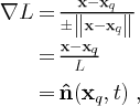
where
![]() denotes a unit vector orthogonal to the LCS at time t. Similarly to above, we also
have
denotes a unit vector orthogonal to the LCS at time t. Similarly to above, we also
have
![]()
So we can now rewrite Eq. (16) as
|
| (20) |
On the LCS, the two points x and xq are equal (and hence L=0); however, we can think of x as a Lagrangian, or material, point which is advected with the fluid, while xq is a point which moves with the LCS. Therefore when evaluated on the LCS, i.e along L=0, the right-hand side of Eq. (20) represents the difference in the velocity of the two points, projected in the direction normal to the LCS. This component of the difference in velocities is precisely what contributes to particles crossing the LCS. Therefore, the total flux across the LCS is given by
|
| (21) |
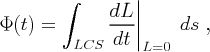
where s is some arc length parametrization variable.
While Eq. (21) presents a concise expression for the flux, by itself it is no more useful than just writing the flux in terms of the right hand side of Eq. (20). Typically when studying a problem we are given the velocity field v, from which we obtain the FTLE field. Therefore, to compute the flux, we should determine

in terms of these two fields (or quantities directly measured from these fields). The following theorem provides such an expression:
|
| (22) |
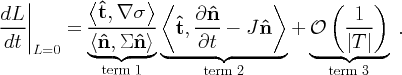
where
![]() is a unit vector tangent to the LCS and J is the Jacobian derivative of the
velocity field v and all terms on the right-hand side are evaluated along L = 0.
is a unit vector tangent to the LCS and J is the Jacobian derivative of the
velocity field v and all terms on the right-hand side are evaluated along L = 0.
The proof of this theorem is somewhat lengthy and will be covered on the next page, however, let us first interpret this result.
- TERM 1
- The factor
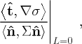
(23) measures how well defined the ridge is, and goes to zero for sharper, well-defined ridges. From Def. 5.1
 evaluated on the LCS must be tangent to the LCS, therefore the numerator
of Eq. (23) can be re-written as
evaluated on the LCS must be tangent to the LCS, therefore the numerator
of Eq. (23) can be re-written as
 .
.For time-independent flows, we will show on the next page that
 is constant along trajectories (asymptotically). Hence for such systems,
along any ridge in the FTLE field,
is constant along trajectories (asymptotically). Hence for such systems,
along any ridge in the FTLE field,
 , and therefore the flux is
zero. This is expected since for time-independent flows, streamlines and
trajectories coincide (e.g. refer back to the double-gyre example
presented earlier). Experience dictates that even for highly
time-dependent flows the value of
, and therefore the flux is
zero. This is expected since for time-independent flows, streamlines and
trajectories coincide (e.g. refer back to the double-gyre example
presented earlier). Experience dictates that even for highly
time-dependent flows the value of
 does not vary much along ridges in the
FTLE
field and hence we can expect
this term to typically be quite small. More precisely though, taking the
derivative of the numerator
does not vary much along ridges in the
FTLE
field and hence we can expect
this term to typically be quite small. More precisely though, taking the
derivative of the numerator
 in the direction orthogonal to the LCS gives
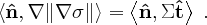
(24) On the next page, we will show that the right hand side of Eq. (24) is zero, a necessary condition for a minimum. Further computation reveals that the numerator in Eq. (23) is indeed a minimum on the LCS.
Referring to Def. 5.1 we notice that the denominator of Eq. (23) is less than zero and is locally minimized (which implies its absolute value is maximized). Therefore, for a well defined ridge, we expect the magnitude of this term to be large, with a larger value the sharper the ridge. Since the numerator of Eq. (23) is locally minimized and the magnitude of the denominator is locally maximized, this implies that the magnitude of the factor given in Eq. (23) is locally minimized in the direction normal to the LCS, hence this multiplying factor is expected to be small for well defined ridges.
- TERM 2
- Now consider the term
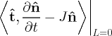
(25) from Eq.(22). The quantity

represents how fast the LCS is locally rotating, which we think of as a Lagrangian rotation. This is easily seen since for an appropriate
 , we can write the unit normal vector
to the LCS as
, we can write the unit normal vector
to the LCS as
and the unit tangent vector as
so
![[ ]
〈 〉 [ ] ˙
∂-ˆn- - θ sin θ
ˆt, ∂t = - sin θ cos θ
θ˙ cos θ
= θ˙ ,](combined221x.png)
which is the local rotation rate of the LCS. Now notice
 is the linearized velocity field applied to a unit vector normal to the LCS;
and taking the inner product of this with the tangent to the LCS,
is the linearized velocity field applied to a unit vector normal to the LCS;
and taking the inner product of this with the tangent to the LCS,
 , gives the component in the direction of the LCS. That is, the term
 measures how much the local Eulerian
field rotates vectors normal to the
LCS. We therefore view this term as a local Eulerian rotation rate and
hence Eq. (25) is a measure of the difference in the rotation rate of
the LCS from the rotation rate induced by the (instantaneous)
velocity field.
measures how much the local Eulerian
field rotates vectors normal to the
LCS. We therefore view this term as a local Eulerian rotation rate and
hence Eq. (25) is a measure of the difference in the rotation rate of
the LCS from the rotation rate induced by the (instantaneous)
velocity field.
- TERM 3
- The last term in Eq. (22) is inversely proportional to the integration time. This tells us that the LCS is more Lagrangian, or behaves more as an invariant manifold, as the integration time T becomes longer.
Most LCS of interest are well-defined, and thus the term (23) is sufficiently small such that the product of terms (23) and (25) is negligible. Additionally, we will see in the Examples that even for relatively short integration times T, ridges in the FTLE field are practically invariant manifolds, with flux measurements on the order of numerical error.
![]()
![]()
![]()