4 How the FTLE is Used

The classical Lyapunov exponent is given by

and is quite useful in the study of Ergodic Theory for time-independent dynamical systems. The seminal works of Lyapunov (1992), Perron (1930), and Oseledets (1968), were very important in laying the theory of Lyapunov exponent, although the manuscript by Barreira and Pensin (2002) contains a good  modern and comprehensive treatment of the subject. However, many dynamical systems of practical importance, especially in the realm of fluids, are time-dependent and only known (either computed or measured) over a finite interval of time. Because of its asymptotic nature, the classical Lyapunov exponent is not suited for analyzing time-dependent dynamical systems or those that are only defined on a finite time interval, so its value is quite limited for practical analyses. Nonetheless, the Finite-Time Lyapunov Exponent is applicable to many time-dependent applications that are perhaps only defined by a discrete data set. The Examples section of this tutorial demonstrates a few interesting applications, furthermore the Additional Reading contains some references to additional applications.

To define a hyperbolic trajectory precisely for systems given only over a finite time interval takes care, e.g. see Haller (1998). However, let us just think of hyperbolic trajectories as ones about which there is a direction of expansion and a direction of compression. In dynamical systems terminology, this means that there should exist stable and unstable directions about a hyperbolic trajectory. For incompressible flows, without sources or sinks, any expansion in one direction must be balanced by compression in another direction, making such trajectories ubiquitous.

Exponential separation between trajectories is to be expected, however if the domain of the system is compact, which is typically the case, these trajectories must mix together. This is especially true for turbulent flows, but even for simple dynamical systems this is also true and is often termed "deterministic chaos", which refers to the phenomenon that even deceptively simple vector fields can produce chaotic trajectories. The structures of strongest hyperbolicity often dictate transport in dynamical systems Ottino (1989), which we will come to see. However, for time-dependent systems these structures, which we refer to as LCS, are often recondite when viewing the Eulerian velocity field or even particle trajectories.

For the remainder of the tutorial, we will assume that , i.e. we only consider planar motion. There is no conceptual difficulty in considering full three-dimensional flows, however the analysis becomes more complicated and is therefore avoided.

To understand how FTLE's can be used to determine LCS, let us consider a simple example, which is given by the following stream function:

over the region D = [0, 2] x [0, 1]. By definition, the vector field is given by

and is plotted in Fig. 6(a). Although this example is time-independent and well defined for all time, its purpose is to provide a simple pedagogical example to start from.

(a) Velocity Field       (b) Streamlines Fig. 6: Panel (a) shows the velocity field of the double gyre example. Panel (b) shows a few streamlines for this flow.

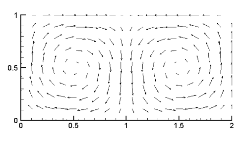
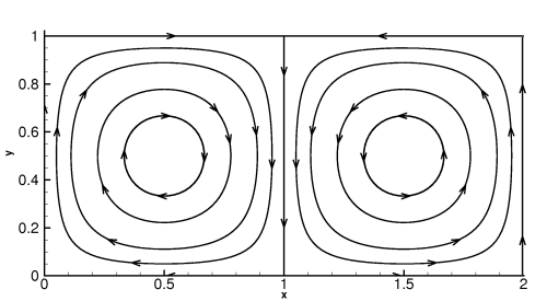
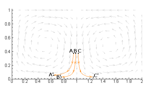
For this example there is a heteroclinic trajectory between the fixed points at (1, 0) and (1, 1). In fact, the boundary of each gyre is composed of heteroclinic trajectories. Heteroclinic trajectories are referred to as separatrices because they separate distinct regions in the flow. As with the pendulum example presented earlier, the double gyre exemplifies this paradigm since these trajectories separate each gyre. Fig. 7 shows the trajectories of three initially close points over a short interval of time. The points B and C are initially close, but since they are located on either side of the separatrix they quickly diverge from each other when advected by the flow. On the other hand, the points initially located at A and B remain relatively close together when advected by the flow.

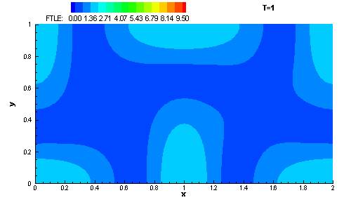
Since points on either side of the separatrix are quickly separated to dynamically distinct regions, this motivates us to believe that the FTLE field should have relatively high values over the separatrix, which turns out to be true. In fact, if we plot the FTLE field for this example, which is shown in the color contour plot of Fig. 8, we notice a very distinguished ridge of high FTLE values along the separatrix. We refer to this ridge of high FTLE values as a Lagrangian Coherent Structure.

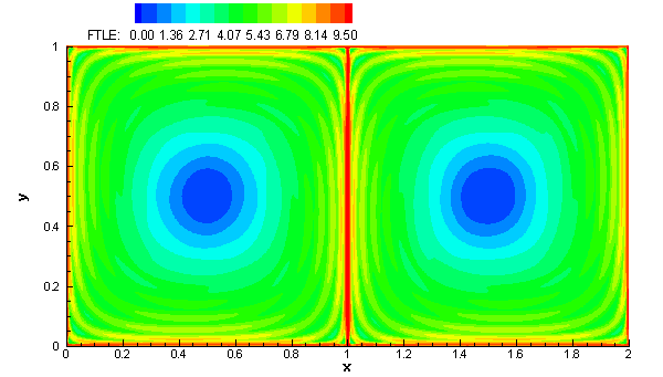
Fig. 8 shows the variation of the FTLE field in space. Since the dynamical system given by (13) is time-independent, the FTLE field does not vary with time, t, however, it is interesting to watch how it varies with integration time T. The movie below shows how the FTLE field varies as T increases from T = 1 to T = 17. 

Next, we will make the definition of LCS using FTLE fields precise. This will allow us to study the properties of these structures more rigorously. Later in the Examples section, we will consider examples much more interesting than the simple one given above, including a time-dependent double gyre, which is similar to the one defined by (13), but with a periodic term included.