3 The Finite-Time Lyapunov Exponent
The finite-time Lyapunov exponent, FTLE, which we will denote
by
![]() , is a scalar value which characterizes the amount of stretching about the
trajectory of point
, is a scalar value which characterizes the amount of stretching about the
trajectory of point
![]() over the time interval [t, t + T]. For most flows of practical importance, the FTLE varies as a function of space
and time. Therefore, one typically is interested in the FTLE
field, in particular how it varies over space and
time. The FTLE is not an instantaneous separation rate like the Okubo-Weiss
criterion, Okubo
(1970) and Weiss
(1991),
but rather measures the average, or integrated, separation between trajectories.
This distinction is important because in time-dependent flows, the instantaneous
velocity field often is not very revealing about actual trajectories, that is,
instantaneous streamlines can quickly diverge from actual particle trajectories.
However the FTLE accounts for the integrated effect of the flow because it is
derived from particle trajectories, and thus is more indicative of the actual
transport behavior.
over the time interval [t, t + T]. For most flows of practical importance, the FTLE varies as a function of space
and time. Therefore, one typically is interested in the FTLE
field, in particular how it varies over space and
time. The FTLE is not an instantaneous separation rate like the Okubo-Weiss
criterion, Okubo
(1970) and Weiss
(1991),
but rather measures the average, or integrated, separation between trajectories.
This distinction is important because in time-dependent flows, the instantaneous
velocity field often is not very revealing about actual trajectories, that is,
instantaneous streamlines can quickly diverge from actual particle trajectories.
However the FTLE accounts for the integrated effect of the flow because it is
derived from particle trajectories, and thus is more indicative of the actual
transport behavior.
To make the expression for the FTLE less obscure, let us
derive it from considering the stretching between two neighboring particles.
Consider an arbitrary point
![]() at time t0. When advected by the flow,
at time t0. When advected by the flow,
![]()
after a time interval T. Since the flow has a
continuous dependence on initial conditions, we know that an arbitrary point near x
at time t0
will behave similarly as x when advected in the flow,
at least locally in time. However, as time evolves,
the distance between this neighboring point and the point x will almost
certainly change. Therefore, let us consider more closely the evolution of a
point close to x, which we will write as
![]() , where we assume
, where we assume
![]() is infinitesimal and, for now, arbitrarily oriented. After a time interval
T, this perturbation becomes
is infinitesimal and, for now, arbitrarily oriented. After a time interval
T, this perturbation becomes
|
(6) |
where the second equality comes from taking the Taylor series
expansion of the flow about point x. Above we employ the
Landau notation, cf. Marsden
and Hoffman (1993).
That is, we write
![]() for a positive function
for a positive function
![]() if and only if
if and only if
![]() remains bounded for all
remains bounded for all
![]() . Since
. Since
![]() is infinitesimal, we can
assume that the
is infinitesimal, we can
assume that the
![]() term is negligible. Therefore,
the magnitude of the perturbation is given by (using the standard vector L2-norm)
term is negligible. Therefore,
the magnitude of the perturbation is given by (using the standard vector L2-norm)
|
(7) |

where we use the convention that M* denotes the adjoint (transpose) of M. The symmetric matrix
|
(8) |
is a finite-time version of the
(right) Cauchy-Green deformation tensor. Note that although
![]() is technically a function of t0, T, and
x, we try to avoid unnecessary notational clutter by simply writing
is technically a function of t0, T, and
x, we try to avoid unnecessary notational clutter by simply writing
![]() instead of, say,
instead of, say,
![]() .
.
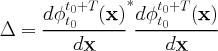
Suppose we are interested in the maximum stretching that occurs between the
points x and y. Notice that this occurs when
![]() is chosen such that it
is aligned with the eigenvector associated with the maximum eigenvalue of
is chosen such that it
is aligned with the eigenvector associated with the maximum eigenvalue of
![]() .
That is, if
.
That is, if
![]() is the maximum eigenvalue
of
is the maximum eigenvalue
of
![]() , thought of as an operator, then
, thought of as an operator, then
|
(9) |
where
![]() is aligned with the
eigenvector associated with
is aligned with the
eigenvector associated with
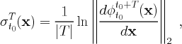
![]() . If we define
. If we define
|
(10) |
then Eq. (9) can be rewritten as
|
(11) |
Equation (10)
represents the finite-time Lyapunov exponent at the
point
![]() at time t0 with a finite integration time T.
at time t0 with a finite integration time T.
Some remarks are in order:
- Remark 1
- The FTLE,
 , is a function of the state
variable x at time t0, but if we vary t0, then it
is also a function of time.
, is a function of the state
variable x at time t0, but if we vary t0, then it
is also a function of time. - Remark 2
- Throughout this tutorial,
 is often referred to as just
 when the extra notation can be
dropped without causing ambiguity.
when the extra notation can be
dropped without causing ambiguity. - Remark 3
- Even though
 is the factor by which a
perturbation is maximally stretched, perturbations often grow exponentially in
time near LCS, which implies that the scaling/normalization introduced in (10)
is better suited for locating such structures. This is especially true when
considering large T and for systems defined on large or unbounded domains, as
is the factor by which a
perturbation is maximally stretched, perturbations often grow exponentially in
time near LCS, which implies that the scaling/normalization introduced in (10)
is better suited for locating such structures. This is especially true when
considering large T and for systems defined on large or unbounded domains, as
 can become numerically
unstable.
can become numerically
unstable. - Remark 4
- It is interesting to note that,
(12) where the subscript in
 explicitly denotes that the L2-norm
is being used, and in this case it's the matrix L2-norm. To see
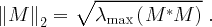
this, we recall that by definition the matrix L2-norm of an
arbitrary matrix M is given by
explicitly denotes that the L2-norm
is being used, and in this case it's the matrix L2-norm. To see
this, we recall that by definition the matrix L2-norm of an
arbitrary matrix M is given by 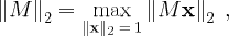
where on the right hand side we are using the standard vector L2-norm. But, following the reasoning above which led to Eq. (9), we have
- Remark 5
- In fluid mechanics, the Eulerian perspective is typically defined as viewing the fluid at fixed points in the domain, perhaps at varying instances in time. When viewing the vector field of a dynamical system, this is typically the standard perspective. On the other hand, the Lagrangian perspective views the flow in terms of particle trajectories. While the FTLE field is technically a Eulerian field, it is thought of as a Lagrangian quantity since it is derived from particle trajectories.
- Remark 6
- Notice that even if the initial perturbation
 is not aligned with the
eigenvector associated with
is not aligned with the
eigenvector associated with
 , the perturbation will
typically align very quickly with this direction. The reason for this is that
if
, the perturbation will
typically align very quickly with this direction. The reason for this is that
if
 has a component in the
eigenvector direction, then this component will quickly dominate because it is
aligned with the most unstable direction.
has a component in the
eigenvector direction, then this component will quickly dominate because it is
aligned with the most unstable direction. - Remark 7
- In the definition of
 in (10),
we used |T|
instead of T because it is often the case that we
are interested in computing
in (10),
we used |T|
instead of T because it is often the case that we
are interested in computing
 for T >
0 and T < 0, to produce LCS akin to
stable and unstable manifolds, as was mentioned towards the end of Sec.
2.
for T >
0 and T < 0, to produce LCS akin to
stable and unstable manifolds, as was mentioned towards the end of Sec.
2. - Remark 8
- The finite-time Lyapunov exponent (FTLE) is sometimes referred to as the Direct Lyapunov Exponent (DLE), a name apparently due to Haller (2001). In this tutorial, we try to stick to the convention of calling it the finite-time Lyapunov exponent, however, we might occasionally refer to the FTLE as the DLE, but know that the two are equivalent.
![]()
![]()
![]()