2 Motivation
A dynamical system in its most general form is often expressed by
|
|
(1) |
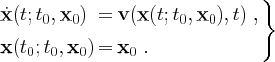
In the differential equation (1),
![]() , represents time and is thought of as the
independent variable, and the
dependent
variable,
, represents time and is thought of as the
independent variable, and the
dependent
variable, ![]() , represents the
state of the system. In some applications, the
domain
, represents the
state of the system. In some applications, the
domain ![]() may be more general than
may be more general than ![]() , but nonetheless we can typically assume that
, but nonetheless we can typically assume that ![]() is a subset of
is a subset of ![]() .
However, many of the results shown in this tutorial can be generalized to more abstract spaces such at tori,
spheres, etc. The vector function
.
However, many of the results shown in this tutorial can be generalized to more abstract spaces such at tori,
spheres, etc. The vector function ![]() typically satisfies some level of continuity. For this
tutorial, let v be smooth. This implies that solutions of Eq. (1)
are smooth and will help relieve us from keeping track of the continuity of
quantities derived from Eq. (1
) or its solutions. This convenient level of continuity is not required, as we
will point out later, but will ease the discussion. As a side note, throughout
this tutorial we will try to denote vector valued quantities by boldfaced letters.
typically satisfies some level of continuity. For this
tutorial, let v be smooth. This implies that solutions of Eq. (1)
are smooth and will help relieve us from keeping track of the continuity of
quantities derived from Eq. (1
) or its solutions. This convenient level of continuity is not required, as we
will point out later, but will ease the discussion. As a side note, throughout
this tutorial we will try to denote vector valued quantities by boldfaced letters.
As time evolves, solutions of Eq. (1)
trace out curves in ![]() , or in dynamical
systems
terminology they
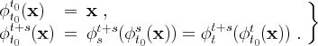
flow along their trajectory. If we fix the initial
time t0 and a (final) time
t, then we can define the
flow map,
, or in dynamical
systems
terminology they
flow along their trajectory. If we fix the initial
time t0 and a (final) time
t, then we can define the
flow map, ![]() , as the map which takes a point in the
domain at time t0 to its location at time
t, i.e.
, as the map which takes a point in the
domain at time t0 to its location at time
t, i.e.
|
|
(2) |
It follows from standard theorems on local existence and uniqueness of solutions, Hartman (1973), of Eq. (1) that the flow map satisfies the following properties:
|
|
(3) |
The underlying motivation for this tutorial is understanding the global flow geometry and transport of time-dependent dynamical systems. Numerical solutions of Eq. (1) can almost always be found by numerically integrating v, however such solutions by themselves are not very desirable for general analysis. Additionally, particle trajectories for time-dependent systems often are convoluted, making it troublesome to study them directly. While the exact solution of Eq. (1) would be ideal, unless v is a linear function of the state x and independent of time t, there is no general way to determine a closed-form analytic solution of Eq. (1).
If v is independent of time t the system is known as time-independent, or autonomous, and there are a number of standard techniques for analyzing such systems. For instance, the global flow geometry of autonomous systems can often be understood by studying invariant manifolds of the fixed points of Eq. (1), in particular stable and unstable manifolds often play a central role.
A fixed point of v is a point xc such that v(xc)=0 . The stable manifolds of a fixed point xc are all trajectories which asymptote to xc when t→∞. Similarly, the unstable manifolds of xc are all trajectories which asymptote to xc when t→-∞. Often, stable and unstable manifolds act as separatrices , which separate distinct regions of motion, making them effective in understanding the flow geometry.
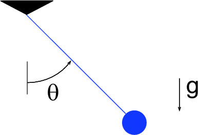
For example consider the planar, frictionless pendulum. This setup has a bob, or point mass, of mass m at the end of a weightless rod of length l, as shown in Fig. 1. Letting g denote the acceleration due to gravity, the dynamics are given by the second order equation
|
|
(4) |
Since any nth order system is equivalent to a first order system, let us define ![]() and
and ![]() , which allows us to write Eq. (4)
as
, which allows us to write Eq. (4)
as
|
|
(5) |
which places it in the first-order vector form given by Eq. (1 ).
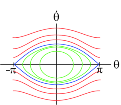
The phase portrait of the pendulum is shown in
Fig. 2.
Since all values for the position ![]() are congruent modulo
are congruent modulo ![]() to a value over the interval from
to a value over the interval from ![]() to
to ![]() , we only show the phase portrait for
, we only show the phase portrait for ![]() ranging over this interval. If we equate positions in
this manner, then technically
ranging over this interval. If we equate positions in
this manner, then technically ![]() is equivalent to
is equivalent to ![]() , however they appear as two separate points in the phase
portrait, but one can reconcile this by mentally wrapping the phase portrait
around a cylinder such that
, however they appear as two separate points in the phase
portrait, but one can reconcile this by mentally wrapping the phase portrait
around a cylinder such that ![]() and
and ![]() meet up. The pendulum has fixed points at
meet up. The pendulum has fixed points at ![]() and
and ![]() . The fixed point
. The fixed point ![]() is
hyperbolic. We will see later that hyperbolicity
plays an important role in transport. The stable and unstable manifolds of the
fixed point
is
hyperbolic. We will see later that hyperbolicity
plays an important role in transport. The stable and unstable manifolds of the
fixed point ![]() are shown in blue in Fig. 2
and form separatrices. These separatrices divide the flow into regions of
distinct dynamics. Inside these separatrices, the pendulum oscillates back and
forth as shown by Animation 3.
Outside the separatrices, the pendulum continually spins in one direction as
shown by Animation 4
.
are shown in blue in Fig. 2
and form separatrices. These separatrices divide the flow into regions of
distinct dynamics. Inside these separatrices, the pendulum oscillates back and
forth as shown by Animation 3.
Outside the separatrices, the pendulum continually spins in one direction as
shown by Animation 4
.
|
|
|
|
The pendulum example helps demonstrate how stable and unstable manifolds can help uncover the global flow geometry of a dynamical system. This is one of the main reasons most introductory texts on dynamical systems dedicate time to explaining such notions and proving their existence. In fact, numerous people have researched different methods for computing, or growing, such manifolds. Many methods rely on growing manifolds from their hyperbolic fixed points. This is possible because for autonomous systems the stable and unstable manifolds of a fixed point are locally tangent to the eigenvectors of the linearized vector field about that point. Hence one can grow these manifolds by cleverly integrating points, which start at a slight offset from the fixed point in an eigenvector direction.
The notion of stable and unstable manifolds becomes ambiguous for time-dependent systems. For example, such systems rarely even have fixed points in the traditional sense, and in addition asymptotic limits for such systems are often meaningless. While there are many academic examples of time-independent dynamical systems, many dynamical systems of practical importance are time-dependent, especially in cases where the dynamical system represents the motion of a fluid.
Surprisingly enough though, even time-dependent dynamical systems typically have regions of dynamically distinct behavior which can be thought of as being divided by separatrices. However, for such systems these regions change over time, and hence so do the separatrices. For a practical example, consider the case of unsteady separation over an airfoil. When the flow over an airfoil separates, there are serious implications to the drag and lift depending on the location of the separation, so this situation is indeed of practical importance (this example will be covered later in Sec. 7.3 ). For this example, the separation profile is a unsteady separatrix which divides the unseparated flow over the airfoil from the "dead-water" zone in which the flow stalls and recirculates.
To find separatrices in time-dependent systems, one might take an approach similar to above and look at fixed points of the instantaneous vector field and try to grow these manifolds by seeding near an instantaneous fixed point and advecting the points according to the time-dependent vector field. While this might seem reasonable, we will see later in the Examples that separatrices in time-dependent flows usually are not connected to instantaneous fixed points, although they might be located nearby. For example, in the case of separation over an airfoil, looking at the instantaneous vector field will predict a separation point (and hence profile) which is noticeably different from the true separation point (and profile).
Instead of trying to directly grow these manifolds, or separatrices, let us try to indirectly obtain them. We will do this by considering the behavior of trajectories near such structures. Our indirect method will spare us from such things as first having to locate fixed points, which can in-and-of itself be a formidable task (plus these points are not typically meaningful for time-dependent systems).
To get us thinking in the right direction, consider a generic hyperbolic point and its associated stable and unstable manifolds, which is depicted in Fig. 5. If we integrate two points that are initially on either side of a stable manifold forward in time, then these points will eventually diverge from each other. Likewise, if we started two points on either side of an unstable manifold, then these points would quickly diverge from each other if integrated backward in time. This is why these manifolds are often called separatrices, since they separate trajectories which do qualitatively different things.
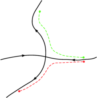
Therefore we take the viewpoint that since separatrices divide regions of qualitatively different dynamics, we can perhaps uncover or define such structures by looking at the divergence or stretching between trajectories. To find separatrices that are analogous to stable manifolds, we measure stretching forward in time and to find separatrices that are analogous to unstable manifolds, we measure stretching backward in time (cf. Fig. 5). However, one should not read into the analogy between these separatrices and traditional definitions of stable and unstable manifolds too much. In fact, since the notions of stable and unstable manifolds are not well defined for time-dependent flows, we refer to theses separatrices as Lagrangian Coherent Structures (LCS), a name which is common is fluid mechanics, but its meaning is often only loosely defined. While there are numerous ways to measure "stretching", we have found that the Finite-Time Lyapunov Exponent provides the best measure when trying to understand the flow geometry of general time-dependent systems.
![]()
![]()
![]()