LCS Tutorial: Flow over an airfoil

7.3 Flow over an airfoil

In this example we show the utility of LCS in obtaining the unsteady separation profile of flow over an airfoil. For most airplanes, separation over the wings is undesirable and leads to stall so airfoils are typically designed to curb such behavior. However, recent developments in the field of aerodynamics have led to the development of airfoils which induce separation very easily. An example of this is the GLAS-II geometry airfoil. This geometry has been used in the area of active flow control where an oscillatory blowing valve is placed on the surface of the airfoil to provide regulated pressure oscillations by means of blowing or suction. This enables control of the separation and reattachment points of the flow over the airfoil, and hence the aerodynamic properties such as lift and drag.

Although for years there has been controversy about how to even define separation, one will likely agree that separation involves the ejection of particles along some path away from a surface. That is, a separation profile should be thought of as a material line (or perhaps surface in 3D) that attracts and ejects particles near the separation point Wang (1982), Haller (2004). Therefore, the separation profile behaves like an unstable manifold. As previously mentioned, for time-independent systems stable manifolds produce ridges in the FTLE field when computed using a positive integration time, T > 0, and unstable manifolds are revealed from backward integration, T < 0.

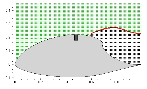
The velocity field over a GLAS-II airfoil was computed from a viscous vortex method Eldredge, et al (2002) and kindly provided by Jeff Eldridge. The flow is actuated to produce a highly unsteady separation point. Locating this unsteady profile is more difficult than locating steady separation. The FTLE field was computed from the velocity data and is shown in Mov. 24 . Again, a bi-colored color map was used such that high values of FTLE are shaded red and low values are white, which allows the LCS to be highlighted, while keeping the rest of the plot transparent. To demonstrate that the LCS represents the separation profile, a uniform grid of fluid particles is placed in the flow at the initial time. Particles initially located above the LCS are colored green, while particles initially located below the LCS are colored black. Note that the trajectories of these particles had nothing to do with the computation of the FTLE field. The location of the blowing valve is denoted by the dark grey rectangle located on the top, center of the airfoil. As we can see from Mov. 24 , even though the LCS is itself highly unsteady, it does a remarkable job capturing the separation profile which divides the unseparated flow from the stalled region behind the airfoil.

Mov. 24: Time evolution of an LCS, given by the red curve, and a grid of fluid particles over a GLAS-II airfoil. In this example, the LCS represents a separation profile that marks the boundary between the free-stream flow from the dead-water zone behind the airfoil.

We should note that the results shown in Mov. 24 are based on rough computations. There are two issues which were neglected. First, in this tutorial we tacitly assume that the dynamical system is void of sources or sinks, at least within the domain for which we compute FTLE's. However, for the flow shown in Mov. 24 there is a blowing/suction valve located very close to the separation point, which is required to produce unsteady separation. Secondly, the integrator which we used to compute the FTLE fields and the particle trajectories shown in Mov. 24 is not symmetric (cf. Ch 5 of Hairer, et al (2002)). Symmetric integrators preserve reversibility, meaning that

Φt+T ∘ Φt = id t t+T

where $Φba$ is the numerical flow from time a to time b, and $id$ is the identity map. Since the FTLE fields were computed from integrating particles backward in time (cf. Sec.8 on The Computation of FTLE) and the particle trajectories shown in Mov. 24 were computed by integrating them forward in time, a symmetric integration should really be used to provide a unbiased comparison. Otherwise, we might expect discrepancies in areas where the flow has large variability, such as near the separation point. However, even with these issues, the LCS shown in Mov. 24 does a very good job capturing the separation profile.

The airfoil example demonstrates that prediction of future Lagrangian behavior can be obtained from FTLE fields computed from integrating backward time. For example, suppose that the initial time at which the FTLE field is shown in the above movie is time t = 3. Suppose that the integration time is T = -3 so that to obtain the FTLE field at time t = 3 we integrate the velocity data from t = 3 to t = 0. We know that the LCS is a quasi-invariant manifold, and varies continually in time assuming the vector field is sufficiently smooth. Therefore we can seed the domain at time t = 3 with a grid of particles and postulate that all particle on one side of the LCS will remain on that side and all particles on the other side of the LCS will stay on the other side when we evolve both forward in time. Of course this should be true of any material line, since any material line is an invariant manifold, however, what makes the LCS special is that it is the material line which separates the free-stream flow from the stalled flow, i.e. it is the separation profile.

Comments, Questions or Concerns can be sent to shawn@cds.caltech.edu