LCS Tutorial: Ocean Currents off the coast of California and Florida

7.2 Ocean currents off the coast of California and Florida

A very interesting application of the theory outlined in this tutorial is for analyzing transport in the oceans. Models of the oceans have been around for years, but recently high-resolution ocean velocity measurements have become available since the introduction of High Frequency Radar technology, which is often referred to as CODAR for COstal raDAR. The examples below make use of such measured data. For more information on how CODAR works, check out this site.

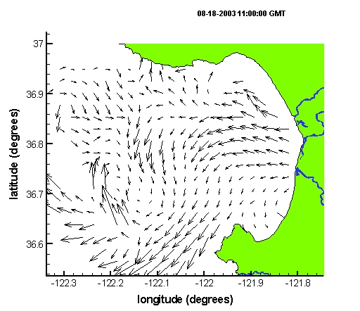
One location that CODAR has been installed is around Monterey Bay, CA. Movie 16 shows CODAR velocity data during August 2003. The data was kindly provided by Jeff Paduan and Mike Cook at the Naval Post Graduate school, which manages the Monterey Bay CODAR system. Notice that this data is highly time-dependent and noisy. This makes it well-suited to "test" the applicability of our theory.

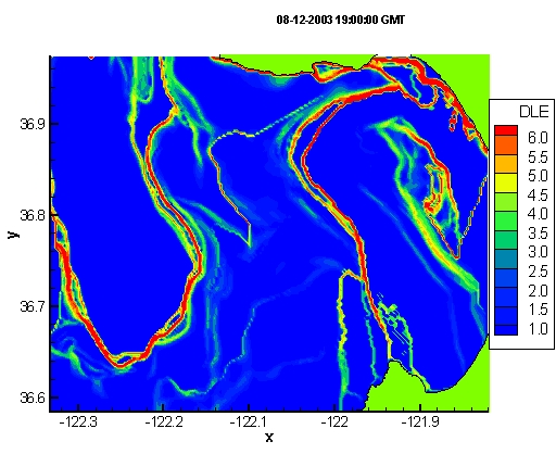
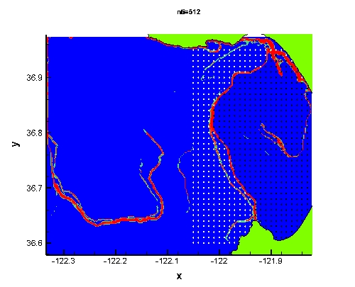
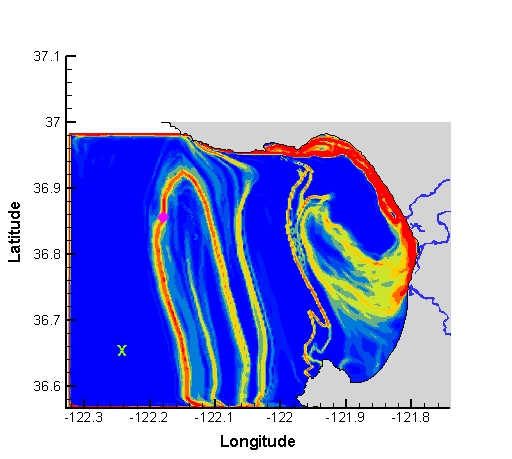
Mov. 16: Velocity data for Monterey Bay, CA during the month of August 2003 obtained by HF-Radar measurements.

Below, we show in Movie 17 the evolution of the FTLE field as computed from the CODAR data. Since our dynamical system is now much more time-dependent, it might be expected that the LCS are more complex. While this is the case, we still see interesting coherent patterns formed by the LCS. For instance, notice that over the time interval shown, there is an LCS which extends across the "mouth" of the bay. This LCS is a separatrix. Particles on the right of the LCS will stay inside the bay and recirculate, while particles to the left of the LCS will continue down the California coast. To demonstrate that this is indeed true, let us choose some arbitrary time and seed the bay with a grid of fluid tracers. We can then superimpose their motion with the motion of LCS. Since we have already compute the FTLE field, let us color the tracers in our grid that initially lay to the right of the LCS black and let us color the tracers that initially lay to the left of the LCS white. We can see from Movie 18 that the black tracers stay inside the bay and recirculate, while the white tracers stay to the left of the LCS and move down along the California coast. (As a side remark, it appears some of the white tracers become stuck near the bottom of the domain. This is because CODAR often produces gaps in the velocity data causing an absence of data for this small area near the coast during the time interval considered, therefore the velocity was simply set to zero at these points, causing the tracers to stop.)

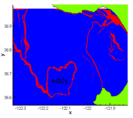
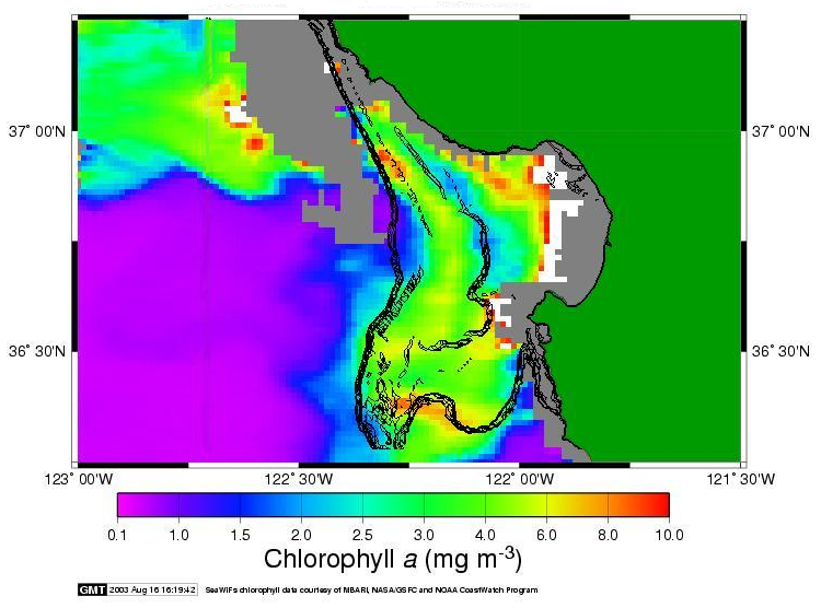
Mov. 17: FTLE field for Monterey Bay, CA

Mov. 18: Evolution of LCS and a grid of fluid tracers. Notice the LCS acts as a separatrix, dividing the flow which stays and recirculates in the bay from the flow which moves down the California coast.

LCS in Monterey Bay often reveal other interesting features. For instance, in Fig. 19 we see an LCS that captures a Lagrangian eddy. Such structures in the flow uncovered by LCS are often completely non-obvious when viewing the Eulerian velocity field or even particle paths. LCS computed in the ocean can be used for a number of interesting applications. For instance, an example of interest might be understanding if pollution released in one area of the ocean will recirculate near the coast, or if it will flush out to open water, as done in the paper Lekien, et al (2004). Another example could be to help understand the transport of plankton, as these organisms are essential to the biological well-being of the ocean. Additionally, it has been shown that LCS can closely resemble fronts in the ocean such as temperature, salinity and even biological fronts; an example of this is shown in Fig. 20, where an LCS (black level sets) is superimposed over a Sea Surface Chlorophyll map taken from satellite.

Fig. 19: Eddy structure captured by LCS in Monterey Bay, CA

Fig. 20: Sea Surface Chlorophyll map with an LCS for the corresponding time superimposed. The LCS is given by the curve of black level sets.

As part of a multi-institutional research effort to better observe and predict the ocean, known as AOSN, LCS have even been used to help understand how one can efficiently sample the ocean with gliders. For example, Movie 21 shows the correspondence between an optimal glider path and an LCS. The glider trajectory was computed independent of the FTLE field. The trajectory is the solution of an optimal control problem, for which the location of the trajectory endpoints were specified and the cost was a combination of the total travel time and the total amount of energy needed. One can see a striking correspondence between the optimal trajectory and the LCS. This application is further explained by Inanc, et al (2005).

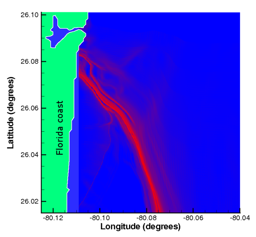
Mov. 21: This movie shows the correspondence between an optimal glider trajectory and an LCS. The purple diamond in the figures near the LCS represents the location of the AUV while the X represents the final target location.

In the paper Shadden, et al (2005), a detailed analysis was performed to verify the flux estimate given by Thm.6.1 on LCS computed from CODAR ocean velocity data. The CODAR velocity data used for that analysis was collected by the Southern Florida Ocean Measurement Center (SFOMC) 4-Dimensional Current Experiment from June 25 through August 25, 1999 Shay, et al (2002).

The FTLE field on July 22, 12:00 GMT is shown in Fig. 22, which has a noticeable LCS extending from the Florida coast. Analysis of the motion of fluid parcels Lekien, et al (2004) reveals that any particle northeast of this structure is flushed out of the domain in only a few hours, while parcels starting southwest of the structure typically re-circulate several times near the Florida coast. Not surprisingly, this behavior is not obvious from observation of the velocity field.

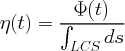
Fig. 22: FTLE field for July 22, 1999 12:00 GMT, computed from SFOMC data (This figure was originally produced by Francois Lekien and reproduced here with his permission).

To verify Thm.6.1, the average flux across the LCS
$Φ(t) η(t) = ∫------------ ds LCS$ (49)

was computed. This was done "directly" by approximating the projected difference in velocity between the LCS and a material line, which corresponds to the LCS at some initial time, using finite differencing. In other words, the LCS is computed for several times $t = t0 + kδt$ , for k = 0, 1, 2,…. In addition, the LCS is advected from time t₀to time t as if it was a line of fluid particles. The difference between the LCS at time t and the integrated line of fluid particles from time t₀to t gives the average flux between the interval from t₀ to t, where t - t₀is the averaging time. As the averaging time goes to zero we expect the measured average flux to converge toward its instantaneous value $η(t)$ .

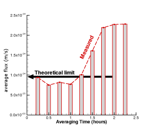
The bars and dashed red line in Fig. 23 represent the "directly" computed rate at which particles cross the LCS as a function of the averaging time. One can see that as the averaging time goes to zero, the rate converges to about 0.0125 cm/s. In addition to computing the flux directly, the first two terms given in Eq. (22) of Thm. 6.1 were computed to first order. This value is referred to as the "theoretical limit" in Fig. 23. Notice that the theoretical limit is very close to the limit of the average flux for the averaging time going to zero. This suggest that the integration time T is long enough for the term $𝒪(1 ∕∣T ∣)$ in Eq. (22) to be negligible.

Not only did the directly computed flux match well with the theoretical flux estimate of Thm.6.1, but notice how small these values are. The typical velocity of fluid particles is about 0.05 degrees/min or 30 cm/s in the vicinity of the LCS Shay, et al (2002). Therefore, the maximum compound flux along the LCS is less than 0.05% of the average speed of the flow in that region! In most cases, this is well below what would be tolerable for numerical error.

Fig. 23: Average flux along the LCS as a function of averaging time; the limiting value for the flux is around $- 4 1.25 × 10$ (This figure was originally produced by Francois Lekien and reproduced here with his permission)

Comments, Questions or Concerns can be sent to shawn@cds.caltech.edu