7 Examples
This section contains various examples of Lagrangian Coherent Structures in time-dependent dynamical systems:
7.1 Time-dependent double gyre
7.2 Ocean currents off the coast of California and Florida
7.4 Lobe dynamics revealed in fluids experiment (coming soon!)
To supplement this section, we will later cover in Sec.8 how FTLE fields computed, so the reader will know how the results shown below are produced. If so desired, Sec.8 on the Computation of FTLE's can be read before this section. Additionally, there is publicly available software, MANGEN, which provides a nice array of tools for analyzing dynamical systems defined by discrete data, including the capability to compute FTLE fields. We will show how to download this software, and walk through the computations shown in Sec.7.3 for flow over an airfoil.
7.1 Time-dependent double gyre
Let's start with an example similar to the double gyre presented in Sec. 4 by Eq. (13). The flow is described by the stream-function
|
| (46) |
where
|
| (47) |
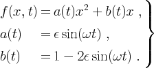
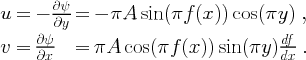
over the domain [0, 2] x [0, 1]. The velocity field is given by
|
| (48) |
For
![]() the flow is time-independent and has the same form as Eq. (13) of Sec. 4.
For
the flow is time-independent and has the same form as Eq. (13) of Sec. 4.
For
![]() the
gyres conversely expand and contract periodically in the x-direction such that the
rectangle enclosing the gyres remains invariant. In Eq. (46), A determines the
magnitude of the velocity vectors,
the
gyres conversely expand and contract periodically in the x-direction such that the
rectangle enclosing the gyres remains invariant. In Eq. (46), A determines the
magnitude of the velocity vectors,
![]() is
the frequency of oscillation, and
is
the frequency of oscillation, and
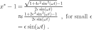
![]() is
approximately how far the line separating the gyres moves to the left or right, that
is, the amplitude of the motion of the separation point
is
approximately how far the line separating the gyres moves to the left or right, that
is, the amplitude of the motion of the separation point
![]() on
the x-axis about the point (1,0) is given by
on
the x-axis about the point (1,0) is given by
|
|
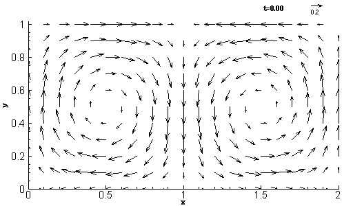
Movie 11 shows the
velocity field of the periodic double-gyre for A = 0.1,
![]() ,
and
,
and
![]() .
Notice that the period of motion is equal to 10 for this case.
.
Notice that the period of motion is equal to 10 for this case.
Recall that for
![]() the stable manifold of the fixed point (1, 0) and the unstable manifold of the fixed point (1, 1) form a heteroclinic connection. Such heteroclinic
connections are unstable and are easily broken by the addition of small
perturbations in time. This leads to classic entanglement of the unstable and stable
manifolds; for references on this behavior see for example Ch.6 of Ottino
(1989) or
Ch.4 of Guckenheimer
and Holmes (1983). This classic entanglement geometry is nicely shown
by the two movies below. However, the perturbation strength, measured
by
the stable manifold of the fixed point (1, 0) and the unstable manifold of the fixed point (1, 1) form a heteroclinic connection. Such heteroclinic
connections are unstable and are easily broken by the addition of small
perturbations in time. This leads to classic entanglement of the unstable and stable
manifolds; for references on this behavior see for example Ch.6 of Ottino
(1989) or
Ch.4 of Guckenheimer
and Holmes (1983). This classic entanglement geometry is nicely shown
by the two movies below. However, the perturbation strength, measured
by
![]() was chosen to be quite large (
was chosen to be quite large (
![]() = 0.25) to demonstrate that the LCS theory is not
restricted to near-integrable systems. In fact, later examples will
show the theory applied to turbulent flows.
= 0.25) to demonstrate that the LCS theory is not
restricted to near-integrable systems. In fact, later examples will
show the theory applied to turbulent flows.
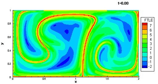
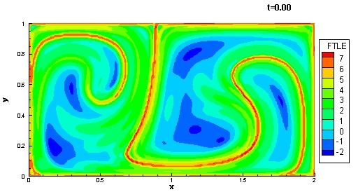
Movie 12(a)
shows the FTLE field computed forward in time with an integration
time length of T = 15. Movie 12(b)
shows the FTLE field computed backward in
time with an integration time length of T = -15. Notice that the flow here is
periodic with period
![]() and therefore the FTLE field is periodic with the same period of motion. Thus, in
Movie 12(a)
the FTLE field
and therefore the FTLE field is periodic with the same period of motion. Thus, in
Movie 12(a)
the FTLE field
![]() is
shown for t = 0 to t = 10 and Movie 12(b)
shows the field for t = 10 to t = 0. In
Movie 12(a)
the ridge in the FTLE field, i.e. the LCS, represents the "stable
manifold" and in Movie 12(b) the LCS
represents the "unstable manifold". Notice that the attachment points
of these manifolds do not correspond to the instantaneous stagnation (fixed) points of the Eulerian
velocity field.
For example, at time t = 0 or time t = 10, the instantaneous fixed
points are located at (1,0) and (1,1), however neither LCS attaches to the
boundaries at these points. This helps demonstrate why trying to "grow"
manifolds from instantaneous fixed points is often troublesome for
time-dependent systems.
is
shown for t = 0 to t = 10 and Movie 12(b)
shows the field for t = 10 to t = 0. In
Movie 12(a)
the ridge in the FTLE field, i.e. the LCS, represents the "stable
manifold" and in Movie 12(b) the LCS
represents the "unstable manifold". Notice that the attachment points
of these manifolds do not correspond to the instantaneous stagnation (fixed) points of the Eulerian
velocity field.
For example, at time t = 0 or time t = 10, the instantaneous fixed
points are located at (1,0) and (1,1), however neither LCS attaches to the
boundaries at these points. This helps demonstrate why trying to "grow"
manifolds from instantaneous fixed points is often troublesome for
time-dependent systems.
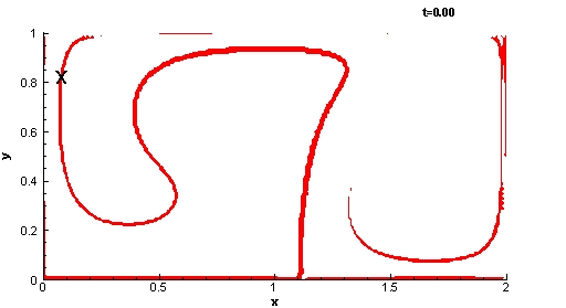
To demonstrate the fact that the LCS shown in Movie 12 are invariant manifolds (or at least quasi-invariant), let us place a material point which moves according to the flow on top of the LCS shown in Movie 12(a). Movie 13 shows the time evolution of the superposition of this material point, denoted by an X, along with the LCS. The initial location of the material point was "eyeballed" to be initially placed on the LCS. From the movie, one can see that the point stays on the LCS when evolved over time. In Movie 13 the LCS is highlighted by plotting the FTLE field using a bi-color contour map in which high values of FTLE's are colored red, and low values colored white. This allows the LCS to be highlighted, and also permits us to better superimpose the evolution of other data. We use similarly skewed contour maps in later examples when showing FTLE fields to help highlight the LCS and keep the rest of the contour plot transparent.
|
|
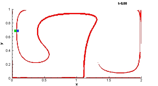
In Movie 14 we now superimpose two parcels of fluid particles, which are initially located on either side of the LCS, with the evolution of the LCS. This movie demonstrates how the LCS acts as a time-dependent separatrix. The parcel which begins to the left of the LCS gets stretched into the left gyre and the parcel that begins on the right side of the LCS gets stretched into the right gyre.
|
|
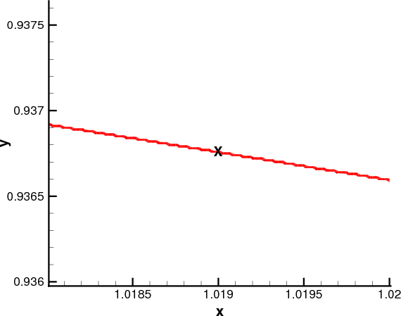
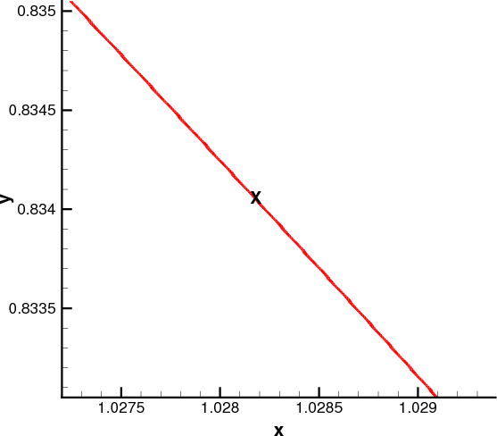
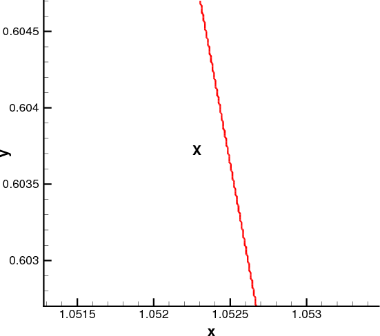
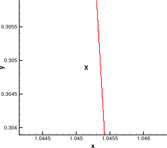
Although the LCS appears to be an invariant manifold from the above movies, we
know from Thm.6.1 that there may be a slight flux across this structure.
Figure 15 shows a
highly refined computation of the LCS and the location of the
Lagrangian tracer shown in Movie 13. The grid spacing that was used for the
computation of FTLE was
![]() .
Computations reveal that the tracer moves at an average rate of
.
Computations reveal that the tracer moves at an average rate of
![]() normal to the LCS over the interval considered. This rate is about 0.05% of the magnitude of the velocity field in that region. This amount is exceedingly small and
well below tolerable numerical error for most practical analyses.
normal to the LCS over the interval considered. This rate is about 0.05% of the magnitude of the velocity field in that region. This amount is exceedingly small and
well below tolerable numerical error for most practical analyses.
To verify Thm. 6.1, the terms in the right-hand-side of Eq. (22)
were computed from a first-order approximation. The
![]() term dominates for this example with
term dominates for this example with
![]() (the other terms of Eq.(22)
are much smaller than 0.03 when evaluated).
The results confirm Eq. (22)
since the "directly computed" flux of
(the other terms of Eq.(22)
are much smaller than 0.03 when evaluated).
The results confirm Eq. (22)
since the "directly computed" flux of
![]() is well below
is well below
![]() .
.
![]()
![]()
![]()