6.3 Proof of flux theorem
This section of the tutorial contains the proof of the flux theorem listed in the previous page. The proof is broken into intermediate results which are listed in theorems, lemmas, etc., which lead to the proof of the flux theorem. Since this page is a little more dense than the others, one can skip this page on a first reading and come back to it later.
Since our flow is Lipschitz continuous, cf. Thm. 1.4 of Verhulst (1996), it satisfies the following condition:
There is a positive constant k such that
|
| (26) |
for all t.
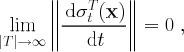
Theorem 6.2 The finite-time Lyapunov exponent becomes constant along trajectories for large integration times T.
PROOF. We compare the value of the finite-time Lyapunov exponent computed at two different points of the same trajectory. Without loss of generality, we assume that the initial time is t0 = 0. Let
![]()
for some arbitrary, but fixed,
![]() .
We have
.
We have
|
|
where we have used properties of the flow map given in Eq. (3) and the maximum exponential stretching hypothesis of Eq. (26). Similarly,
|
|
so we have
|
| (27) |
Therefore
|
| (28) |
Taking the limit as
![]() gives
gives
|
| (29) |
which implies
|
| (30) |
■
The following Corollary provides a bound on the variation of
![]() in
time.
in
time.
PROOF. From Eq. (28)
![]()
As a result,
|
| (32) |
Taking the (spatial) derivative of this equation yields
|
| (33) |
assuming that
![]() ,
,
which is reasonable since
![]() is smooth since the flow is assumed to be smooth.
is smooth since the flow is assumed to be smooth.
■
Let
![]() be
the Hessian of
be
the Hessian of
![]() and note the following properties of
and note the following properties of
![]() and
and
![]() :
:
Lemma 6.1
![]() and
and
![]() are self-adjoint.
are self-adjoint.
PROOF. This result holds due to the symmetry of mixed partials. For example,
from
![]() , we
deduce immediately that
, we
deduce immediately that
![]() because the derivatives are necessarily real numbers.
because the derivatives are necessarily real numbers.
■
PROOF. From Def. 5.1, SR2 implies that
![]() is
an eigenvector of
is
an eigenvector of
![]() .
Hence,
.
Hence,
![]()
since by definition the two vectors are orthogonal, where
![]() is
the smallest eigenvalue of
is
the smallest eigenvalue of
![]() .
.
■
PROOF.
Developing v in
the orthonormal basis
![]() gives
gives
|
| (34) |
A direct computation of
![]() ,
and applying Thm. 6.3, gives the desired result.
,
and applying Thm. 6.3, gives the desired result.
■
PROOF. Everywhere in U, L is
smooth and the gradient
![]() is well-defined. In particular, from Eq. (19)
is well-defined. In particular, from Eq. (19)
![]() ,
therefore
,
therefore
|
|
(35) |
■
|
|
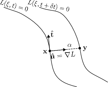
PROOF. Take x on
the LCS at time t, i.e.
![]() . Define
. Define
![]() such that
such that
![]() . In
other words, y is
at the intersection of the LCS at time
. In
other words, y is
at the intersection of the LCS at time
![]() and the line starting at x,
orthogonal to the LCS at time t (see Fig. 10). Since we require y
= x
for
and the line starting at x,
orthogonal to the LCS at time t (see Fig. 10). Since we require y
= x
for
![]() , it
follows that
, it
follows that
![]() is
is
![]() .
Expanding L to
second order in
.
Expanding L to
second order in
![]() gives the following (where all derivatives on the right-hand side of Eqs. (37)–(41)
are evaluated at x and t unless otherwise specified):
gives the following (where all derivatives on the right-hand side of Eqs. (37)–(41)
are evaluated at x and t unless otherwise specified):
|
| (37) |
Therefore,
|
| (38) |
Now expanding
![]() ,
and plugging in Lem. 6.2, gives
,
and plugging in Lem. 6.2, gives
|
| (39) |
From Eqs. (19) and (38) we have
|
| (40) |
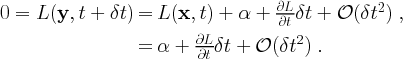
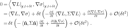
Since y is
on the LCS at time
![]() , we
must have
, we
must have
|
| (41) |
Hence, we get the desired result, since
![]() is
arbitrary.
is
arbitrary.
■
We now have all the precursors to prove Thm. 6.1, which we have restated below for convenience.
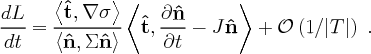
PROOF. Lemma 6.3 gives
|
| (43) |
Applying Cor. 6.2 and the chain rule for the derivative gives
|
| (44) |
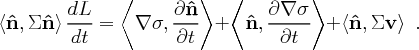
Using Cor. 6.1 in Eq. (44) gives
|
| (45) |
and the result follows by noticing that for L = 0,
![]() is
proportional to
is
proportional to
![]() ,
hence
,
hence
![]() .
.
■
![]()
![]()
![]()