8 Computation of FTLE
This section provides an overview of the numerical computation of FTLE's and LCS and a few computational concerns. Of course in practice, there are a number of numerical issues to worry about when running such computations, but the objective here is to focus on the main points. To put the computational algorithm into context, we use the airfoil example of Sec.7.3 to help illustrate the steps.
For many practical applications, the dynamical system is given by a discrete set of data, which is often obtained from fluid dynamics computations or from direct measurements. For the flow about the GLAS-II airfoil described in Sec.7.3, the velocity field was computed from a Computational Fluid Dynamics (CFD) simulation. We have animated this data in Movie 25 .
Suppose we are interested in computing the FTLE
field, ![]() , over the airfoil at say time
t = 8. Since we can only compute the field at
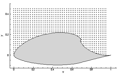
discrete points, we first choose a discrete grid of points over which we want
to compute the value of
, over the airfoil at say time
t = 8. Since we can only compute the field at
discrete points, we first choose a discrete grid of points over which we want
to compute the value of ![]() , cf. Fig. 26
.
, cf. Fig. 26
.
Recall that the FTLE is given by
|
|
(50) |
where
|
|
(51) |
To compute the FTLE at each point in our grid, x, we must obtain the
flow map ![]() at each point. That is, we must compute the position
at each point. That is, we must compute the position ![]() of each point when advected by the
flow for a amount of time
T. To obtain this, each point is advected with a
4th-order Runge-Kutta-Fehlberg integration algorithm using the provided
velocity data. For discrete velocity data, a 3rd-order interpolation Lekien
and Marsden (2005)
is typically used to provide necessary interpolation. Numerically integrating
vector fields is very basic to applied dynamical systems, and is discussed in
any book on numerical methods for differential equations.
of each point when advected by the
flow for a amount of time
T. To obtain this, each point is advected with a
4th-order Runge-Kutta-Fehlberg integration algorithm using the provided
velocity data. For discrete velocity data, a 3rd-order interpolation Lekien
and Marsden (2005)
is typically used to provide necessary interpolation. Numerically integrating
vector fields is very basic to applied dynamical systems, and is discussed in
any book on numerical methods for differential equations.
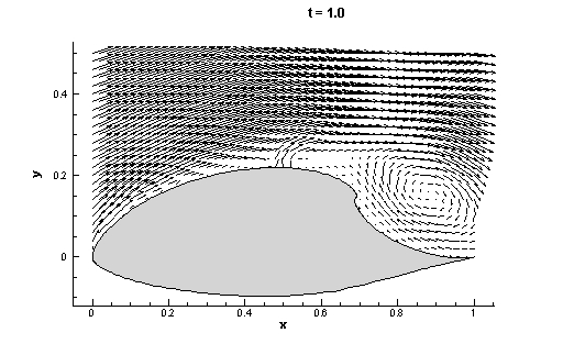
Recall that for the airfoil example, the FTLE fields were computed by integrating backward, i.e. T < 0. This is because the separation profile is an attracting coherent structure, and such LCS are obtained from backward integration. Movie 27 shows the integration of the grid from t = 8 to t = 7, which might correspond to choosing T = - 1. We will later comment on how the integration length |T| should be chosen.
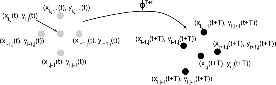
Once we have mapped the points in our grid from their initial positions, x(t) , to their final positions x(t+T), we must compute the gradient of the flow map. Assuming that points in the grid are initially close enough together, we can compute the gradient of the flow map from finite differencing. For example, the formula for the gradient of the flow map at an arbitrary point in our grid, which we will denote point (i, j), using central differencing would be
|
|
(52) |
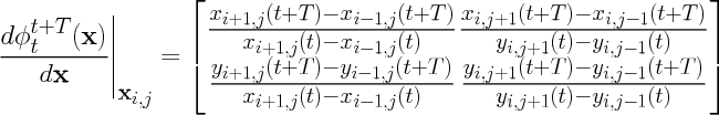
where we use the convention that ![]() are the coordinates of point (i, j)
at time
t, see Fig. 28
.
are the coordinates of point (i, j)
at time
t, see Fig. 28
.
Once we have computed Eq.(52)
for each point in our grid, we can left multiply this matrix by its transpose
to obtain ![]() at each point. Then we simply compute the largest eigenvalue of
at each point. Then we simply compute the largest eigenvalue of ![]() (which is rather trivial for
(which is rather trivial for ![]() matrices) and plug into the formula for the FTLE given by Eq.(50).
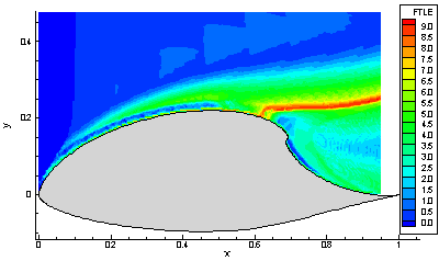
Doing this for each point in the grid gives the FTLE field. This data can then
be visualized, for example by a color contour plot. One program that is good
for visualizing data is Tecplot, which is the
visualization tool that was used to create many of the figures and movies shown
in this tutorial. Figure 29
shows the color contour plot of the FTLE field above the airfoil computed at
t = 8 using a uniform grid with a spacing of 0.01
in both the x- and y-directions and an integration time of
T = -
4.
matrices) and plug into the formula for the FTLE given by Eq.(50).
Doing this for each point in the grid gives the FTLE field. This data can then
be visualized, for example by a color contour plot. One program that is good
for visualizing data is Tecplot, which is the
visualization tool that was used to create many of the figures and movies shown
in this tutorial. Figure 29
shows the color contour plot of the FTLE field above the airfoil computed at
t = 8 using a uniform grid with a spacing of 0.01
in both the x- and y-directions and an integration time of
T = -
4.
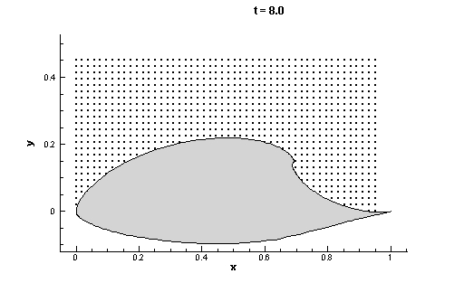
The above procedure gives the FTLE field (over a discrete grid) at the time t = 8. This procedure can be repeated for a range of times t to provide a time-series of FTLE fields. Once FTLE fields have been computed in this manner for a series of times t, the forward time evolution of the these fields (and hence the LCS) can then be presented by sequentially showing these fields as t increases, for example this was done to produce Movie 24 .
One question that still looms is, how is the integration length |T| chosen? The choice of integration length is dependent on the particular application, as one might expect. In general, the longer |T| is, the more refined the LCS become. However, for dynamical systems defined by discrete data, probably the most important indicator of what |T| should be is how long it takes for particles to exit the domain. For example, the velocity data for the airfoil is shown in Mov. 25. This data is given over the rectangular domain [0, 1] x [0, 0.5]. Since we do not know the velocity field outside of this domain, it is not feasible to integrate particles outside of this region. If we consider the grid shown in Fig. 26 and its evolution shown in Movie 27 we notice that many particles leave the domain in less than 1 second. Since we do not know the evolution of these particle after they leave the domain, we must evaluate Eq.(52 ) using the position of each point prior to its exit as the final position value. Therefore, if nearly all points in our FTLE grid leave the domain in say 4 seconds, then it doesn't make sense to choose |T| > 4, since further integration would not change the FTLE field any. Alternatively, the duration of available data might be the limiting factor. For instance, if we are only given 10 seconds of velocity field data, then it not feasible to choose an integration time longer than 10 seconds.
For the time-dependent double gyre presented in Sec.7.1, the boundaries of the domain [0, 2]x [0, 1] are invariant manifolds, so particles will stay inside this domain for all times. Additionally, the vector field is well-defined for all times. Therefore we do not run into the problems stated in the paragraph above. In this case we can choose |T| as large as we want. The effect of increasing |T| will be to further refine the LCS. For example, in Mov. 30, we show the variation of the FTLE field for the time dependent double gyre as T increases from T=1 to T=22. Notice that as T increases, the LCS grows and further looping is revealed. Therefore increasing the integration time is analogous to growing the manifold, as done in other techniques used to determine invariant manifolds (which are typically only suited for time-independent systems). This behavior should be expected after referring back to the cartoon in Fig.5. If the two points shown in that figure started "further up" the manifold (i.e. to the right) then they would take longer to separate, and hence a longer integration time is needed to "grow" the manifold. This quality even carries over to time-dependent systems where the LCS is not even attached to a fixed point. However one must be careful to not select |T| too large. Recall that in Sec.3 we assumed that the stretching between two neighboring points is governed by the derivative (linearization) of the flow map. This assumption is valid assuming the initial separation is infinitesimal. However, in computations, there is always a finite distance between points in our grid, so the assumption of only needing the linearization of the flow map breaks down as |T| increases. Therefore if one is to choose a large integration time |T|, then the grid spacing should be sufficiently small.
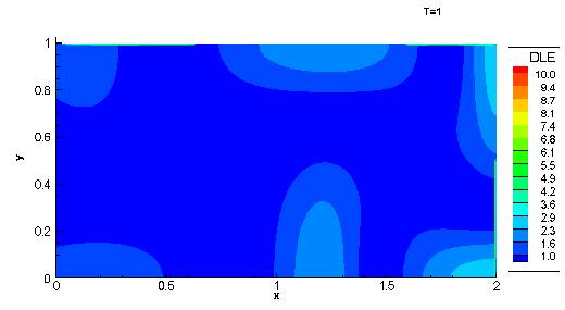
| Mov. 30: | Variation of the FTLE field for increasing integration time T. Notice as T increases, further looping of the LCS is revealed |
![]()
![]()
![]()