9 MANGEN
A software package, known as MANGEN for MANifold GENorator, was originally created at the California Institute of Technology by Francois Lekien and Chad Coulliette and provides a set of tools for analyzing dynamical systems. A nice capability of this software is the ability to easily load velocity field data sets and quickly initiate FTLE calculations. MANGEN is publicly available and is archived in the following zip or gnu zipped tarball files.
Below, we show how MANGEN can be used to produce the FTLE fields shown in Movie 24 . To visualize the results, it is strongly recommended that Tecplot be used, as MANGEN outputs data in an ASCII format which is structured to be read by Tecplot. As a precaution, MANGEN does contain bugs and limitations that users need to be aware of if they intend to seriously use this software, however for the purposes of completing the example computations below, these issues should not interfere.
Windows Users:
For the Windows' version, there is a convenient GUI which can be used to configure computations.
- Step 1
- Click here to download the zipped file and unzip to a directory of your choice. Additionally, click here to download the input files needed for the airfoil example and unzip them as well.
- Step 2
-
Run the program mangen.exe by double-clicking on it. You will get a display
like the one shown below:
- Step 3
- Go to the File menu and select Open... and open the airfoil.in file that was contained in the zip file you downloaded. Once MANGEN opens the file, it will display some warning messages, just click on the ok button.
- Step 4
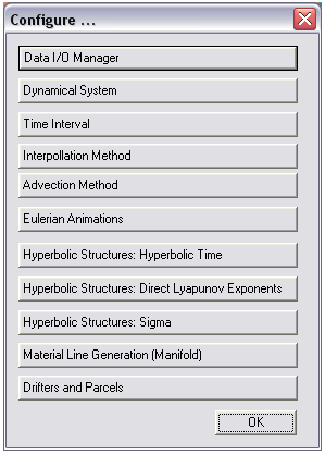
- Go to the Simulation menu and click Configure... . You will get the following menu which lists all the features that MANGEN supports:
- Step 5
-
Click the
Data I/O Manager
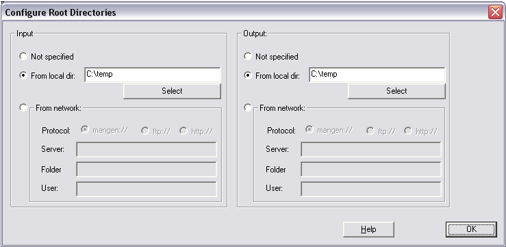
button. You will get a the following display:
Change both of the From local dir: text edit fields from C:\temp to whichever directory you unzipped the MANGENfiles.zip file into. Then click the ok button. From this point on, we do not need to change anything else before we run the computations. However, we will explain the remaining parameters that have already been set for the computation to run.
- Step 6
-
Click the
Dynamical System
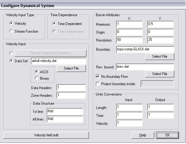
button in the Configure menu. The following display will appear:
Some items that are worth noting are
- The Velocity Input section is where the dynamical system is specified. We have the ability to specify an analytical equation for the vector field or we can input the vector field from a data set, which is the case for the airfoil problem we are studying. The velocity field for the airfoil is contained in the file airfoil-velocity.dat. This data is ASCII formatted, so one can view the file with a standard text viewer or editor. The structure of the data in that file is set up to be read by Tecplot. Therefore if you have a copy of Tecplot, you can simply open the file airfoil-velocity.dat in Tecplot and plot the velocity field. Of course, if you do not have Tecplot but still want to plot the velocity field with your program of choice, then you must convert the file airfoil-velocity.dat to a format which can be interpreted by that program.
- The Basin Attributes section specifies the domain of the velocity data and specifies the resolution of the data as well (these are not needed if an analytical vector field is being used). This section also contains a field to input boundary information. For the airfoil, the closed boundary is given by the surface of the airfoil, which is specified by the file topo-comp-GLASII.dat. If we to make sure points are not advected through this boundary, then we check the No Boundary Flow check box.
- The Units Conversions section allows multiplying factors to be added to the input data in case the data which is being input is not in consistent units, or not in units that are well-suited to keep numerical errors low.
When done viewing the Dynamical System configuration GUI, click the ok button.
- Step 7
-
When selecting the
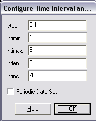
Time Interval
button from the Configure menu, you get the GUI given in
Fig. 34.
The file airfoil-velocity.dat contains velocity data from
t = 1 (sec) to
t = 10 (sec) at time steps of 0.1
(sec). Therefore, there are 91 "zones", or time slices, of data
contained in our input file. The value in the
step
field specifies that the time spacing between zones in our data file is
0.1 and the
ntlen
field specifies that there are a total of 91 time slices of data. The
values
ntimin
and
ntimax
specify the duration over which we want to
perform our computations, whatever they may be.
The values of
ntimin
and
ntimax
are set to 1 and 91 respectively, which means that the computations will
span the entire length of data we have available. The last value which can be
specified is
ntinc, which is a boolean value that is
set to 1 if computations are to be carried out forward in time and set to -1 if
computations are to be carried out backward in time. For the airfoil example,
recall that we want to compute the FTLE fields
with a negative integration
time,
T < 0, which is why
ntinc
is set to -1. When done viewing this menu, press the
ok button.
- Step 8
- The Interpolation Method and Advection Method menus are fairly self-explanatory. They allow the user to specify the method used to interpolate the velocity data, and the method used to integrate the velocity data.
- Step 9
-
The remaining buttons in MANGEN's
Configure... menu specify what
computations should be performed. Since we are only interested in computing
FTLE fields, the only menu that is of interest is the
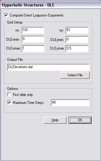
Hyperbolic Structure: Direct
Lyapunov Exponents
menu (recall the phrase Direct Lyapunov Exponents is synonymous with
Finite-Time Lyapunov Exponents). After pressing this menu button the GUI given
by Fig. 35 will
appear. The
Grid Setup
fields allow the user to specify a cartesian mesh over which the FTLE
field will be computed, cf. Fig
26. The values
nx
and
ny
specify the x- and y-resolution, respectively, of the mesh. Once FTLE
fields have been computed, they will be saved to the file specified in the
Output File
text edit box. For this example, we will compute FTLE as a function of
time, so we will leave the
First slide only checkbox unchecked. The
Maximum Time Steps
input field allow the user to specify the integration time length, i.e.
|T| (note
that it is the absolute value of
T because the sign of
T is determined by value of
ntinc
given in the
Time Interval configuration menu). A value
of 40 indicates that
|T| should
be 40 time slices long, and since each time slice in the input file
airfoil-velocity.dat is spaced every 0.1 (sec), then a value of 40 time slices
is equivalent to an integration length of 4 (sec). If the
Maximum Time Steps
checkbox is left unchecked, then MANGEN will integrate the FTLE's using
the largest possible integration time length. When done viewing this menu,
press the
ok button.
- Step 10
-
The last thing left to do is to start the computations. Close the
Configure menu if you haven't already done
so, and it would probably be wise to save the changes you've made to
airfoild.in by going to the
File
menu and selecting
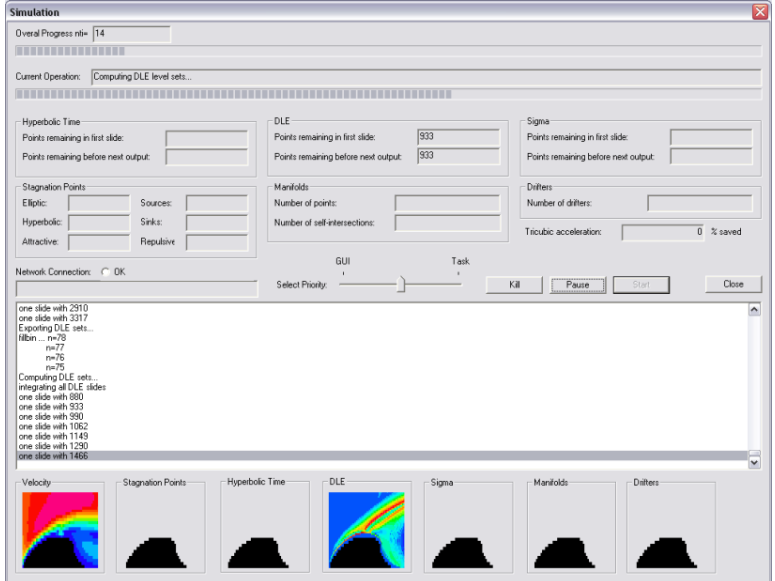
Save. To start the computations, simply go
to the
Simulation
menu and select
Start. This will bring up the simulation
monitor GUI. Click Start and the computations will (hopefully) begin.
The first thing that MANGEN will do is convert the airfoil-velocity.dat file
into a binary. If you re-run any computations using this velocity data, it is
best to use the binary file airfoil-velocity.dat.man as the input instead of
the ASCII file. Once you tell MANGEN that it is ok to convert the ASCII
file to a binary, MANGEN will begin to compute FTLE's. The simulation monitor
GUI will continually update its display to show you the progress of the
computations, and will look something like Fig. 36.

- Step 11
- Once the simulation is finished, the file DLElevelsets.dat should contain the finite-time Lyapunov exponent data. Since the data is in ASCII format, one can view the contents in any text editor. The layout of the data is setup to be read by Tecplot so one can easily plot the FTLE fields by loading this file to Tecplot and viewing as a contour map.
Linux (and perhaps Mac) Users:
- Step 1
- Download the MANGEN source tar file from http://www.mangen.info/mangen-latestversion.tgz and uncompress the files. Additionally, click here to download the input files needed for the airfoil example and unzip them as well.
- Step 2
- After untarring the source files, in the \source\UNIX directory there is a README file that contains instructions for compiling the source code and running MANGEN. Follow the instructions to compile the code. If using the configure script, one might need to change it to an executable by typing chmod ugo+x source/UNIX/configure
- Step 3
- Now we need to edit the airfoil.in file which specifies all the parameters that need to be set for our computations. For the Windows version of MANGEN, there is a convenient GUI which allows the user to configure all parameters for the computation (see above). However, this GUI is basically a glorified editor for the MANGEN input file, which in this example is the airfoil.in file. When running the Linux version of MANGEN, one does not have the convenience of the GUI, but rather has to manually edit the .in file. All that needs to be changed in airfoil.in to run the computations are the values for inprefix and outprefix, which are the first two variables that are listed in the input file. Therefore, open the file airfoil.in in your favorite text editor and change the values of inprefix and outprefix from C:\temp to the directory which contains the input files (airfoil.in, airfoil-velocity.dat, and topo-comp-GLASII.dat) and save. The airfoil.in file is well commented, so the file should be quite self-explanatory. If you are interested in knowing what other variables are required to run the computation, please refer to the Windows Users explanation above, or browse the file, however everything else is already set to run the computations so nothing else should be changed.
- Step 4
- Start the computations by typing mangen airfoil.in on the command prompt
- Step 5
- Once the simulation is finished, the file DLElevelsets.dat should contain the finite-time Lyapunov exponent data. Since the data is in ASCII format, one can view the contents in any text editor. The layout of the data is setup to be read by Tecplot so one can easily plot the FTLE fields by loading this file to Tecplot and viewing as a contour map.
![]()
![]()
![]()