6 LCS Properties
The purpose of this section is to show whether LCS represent time-dependent invariant manifolds, and derive a few interesting intermediate results. This section is broken down into three subsections:
To summarize, we show that for well-defined LCS, which are obtained from FTLE fields with a sufficient integration time |T|, the flux across such structures is expected to be small. This should seem intuitive since one might expect that very faint ridges in the FTLE field are less Lagrangian than those that are well-defined. Additionally, recall that the FTLE measures the integrated effect of the flow, so if |T| is too small then this integrated effect is ignored and thus the FTLE is not very indicative of Lagrangian behavior. However, we will see in the Examples section that LCS (at least the ones which are clearly visible in the FTLE fields) are invariant for all practical purposes.
The theorem which states the exact estimate for the flux over an LCS is given by Eq. (22) in Sec. 6.2. Arriving at this expression is somewhat lengthy. If you would rather accept the paraphrase in the previous paragraph and go on to see LCS "in action" then you might want to skip this section to continue to the Examples section and return to this section when desired.
6.1 LCS Representation
Our motivation is to determine if LCS are invariant manifolds. To resolve this we will derive an estimate for the flux through an LCS based only on the FTLE field and quantities defining the LCS. To facilitate the derivation, let us choose a function L(x, t) such that the LCS is given by the zero level set L(x,t)=0.
Suppose we are given a (perhaps time-dependent) FTLE field which admits an LCS, as defined in Def. 5.2. For every time t, let L(x, t) be defined by the conditions
- L1
-
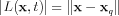
, where xq is the point on the LCS closest to the point x.
- L2
-

where
 is the unit basis vector
pointing "up" from the domain
is the unit basis vector
pointing "up" from the domain
 .
.
The definition for L(x, t) looks a little confusing but it simply just gives the "signed distance" from an arbitrary point x in the domain to the nearest point on the LCS (part L1 gives the distance and part L2 gives it a plus or minus sign depending on what side of the LCS it's on). If moving along the LCS curve c(s) in the positive c'(s) direction, then at least locally, points on the right have a positive value of L, and points on the left a negative value, and importantly the LCS is given by the zero set L=0. While L is not explicitly a function of time, at least as defined in L1 and L2, we write L(x, t) above to emphasize that L does indeed vary with time, although it is through the dependence on xq, which is time-varying .
![]()
![]()
![]()